Last December the 10th in Barcelona we were happy to present the first  Brainpolyphony Orchestra Concert. Brainpolyphony is a project born thanks to the collaboration of CRG, University of Barcelona and Starlab with the goal of giving voice, or in this case music, to people with severe communication difficulties.

Patients with neurological diseases such as cerebral palsy often experience severe motor and/or speech disabilities that makes very difficult (and in some cases even not possible) for them to communicate with their family and carers. We believe that a possible solution to overcome these communication difficulties is to develop a Brain Computer Interface (BCI) system that uses robust reliable electroencephalographic patterns. Since emotions play a crucial role in daily life of human beings, we believe that emotional changes monitoring would be the best communication approach. The platform works as a dictionary of emotions, detecting patterns from emotional states (rythms from electrical brain activity) and translating them into (emotional) sound; thus making the user/caregiver a new tool to understand those signals in a direct way.

Data sonification is the process of acoustically presenting information. Sonification intends to take profit of specific characteristics of the human sense of hearing (higher temporal frequency and amplitude resolution) compared to vision. Most of the work done in rehabilitation using sonification techniques has been conducted among visually impaired people, however the potential of sonification for offering channels of communication to persons with restricted capacities has great possibilities in the field of assistive technologies. Following this line Brainpolyphony uses sonification of emotions as communication vehicle for cerebral palsy patiens. In its musical composition module, emotional information is used to create in real time a unique theme, following musical rules, that reflects the user emotional state. In example, if the person using the Brainpolyphony system starts feeling sad, the music coming out of the platform will be unequivocally gloomy and melancholic.

Using the first prototype three volunteers with cerebral palsy: Marc, Merce and Pili came onto stage. Ivan Cester, our composer, specialized in movies sound-tracks and jingles, created a new online musical composition (using Max Studio) that changed the melody upon the received level of real-time streamed volunteer’s emotional information. The three volunteers were looking at a set of videos with strong emotional content in order to make their emotional signature change during the performance. As result the three of them created a unique dynamical musical composition based on their measured emotions. Sant Cugat Young Orchestra improvised with them creating an incredible experience!.

But it is better to see it in action. In the following videos you can see (and listen to) Marc, Pili and Mercé who are looking at the videos with the orchestra behind them. However there is still a long way to go as this was a proof of concept of the very first prototype. We hope to develop in the following years a reliable, customized, affordable solution that could improve the quality of life of many people with severe communication problems.

We all think, we all talk, we all communicate and navigate this world but we barely take some time to watch and observe the signals that come out of our own brain. This time, Starlab® and Neuroelectrics® have worked together to develop a brain monitoring and experimental setup within the exhibition of the TalkingBrains, powered and designed by Indissoluble.

The TalkingBrains exhibit, currently at the CosmoCaixa in Barcelona, aims to provide a scientific approach to language processing, emphasizing its variability across society, genetic determinants or its evolution through humans and non-human primates.

Do you want to contribute to current scientific research? Do you want to see and share your own brain activity? Visit CosmoCaixa in Barcelona! 

What is human language? What does it mean? When and where does it appear? How do scientists study language? Humans have the ability to communicate through language, spoken or signed in a way that projects our thoughts to the world, facilitating communication and interaction between the external world and us. But, when and how did we develop this ability? These and many other questions are addressed at the TalkingBrains, where diverse aspects of language are explored.

From Starlab®, we wanted to contribute to this exhibit by providing the tools that would allow for the exploration of the physiological basis of language. How does the brain process language? The brain communicates through electrical signals that can be monitored through surface sensors, like the ones in our electroencephalographic (EEG) wireless monitoring system. This system allows for the visualization of your brain activity, displayed for you and your colleagues to watch and observe the signals that come out of our own brain. Visitors that accept to participate in the installation would actually be conducting tasks associated to language – like sentence comprehension and memorization – and would get the chance to visualize their brain activity!

Our installation would not only explore the physiological basis of language, it would also allow participants to take part in a scientific campaign by the UPF and Starlab®. The exhibit has been designed to monitor and record brain signals associated to the language experiments you will be conducting, which will allow us to test two scientific hypotheses. Which ones? Come and visit CosmoCaixa in Barcelona to find out!

Indissoluble.

Javier Acedo, Marta Castellano and Jordi Prados -
 Marta Castellano

Marta Castellano

Indissoluble.

Indissoluble.

Science is advancing in Catalunya, which is reflected through the creation of RIS3CAT communities. These communities arise from a new EU-funding program (ERDF), a fund that aims to develop R&D projects and support the association between diversified entities for the advancement of the society.

Our community, called NextHealth, encloses a group of entities that work on multidisciplinary solutions for upcoming health challenges, coordinated by Biocat. The NextHealth community aims to resolve health challenges through the financing of 5 projects, each of them implicating a tight collaboration between hospitals, public research institutions and companies. This partnership between diverse entities connects the bench to the hospital, aiming to directly integrate R&D advancements into the Catalan health system. Projects within the NE community are highly innovative both economically and socially; aiming to solve specific health challenges and the Catalan health system, to strengthen collaboration and competitiveness of participating entities, and to identify and boost new commercialization opportunities in the health domain.

The Ris3cat|Nexthealth community after the 1st General Meeting at the University of Barcelona, Faculty of Medicine (copyright: Biocat).

Innobrain aims to provide new technologies for innovation in rehabilitation and cognitive stimulation through the consolidation of the NeuroPersonal Trainer platform, developed by the Guttmann Institute. To this date, the platform provides a framework for cognitive rehabilitation and stimulation for people with cognitive deterioration or cognitive deficits, appearing either as a result of a neurological disease, dementia, psychiatric conditions or developmental disorder. This tool aims to improve the health care of these populations at risk by personalizing cognitive training protocols as defined by professional experts in neuropsychological assessment.

With our passion in cognition and cognitive rehabilitation, Starlab joins the Guttmann Institute with the goal of contributing to increase the efficacy and efficiency of the cognitive rehabilitation strategies. We are providing our strength: the in-house knowledge on electrophysiological monitoring technologies as a physiological marker of neurological disease, dementia, psychiatric cognition or developmental disorders, along with an enthusiastic fascination towards cognitive processes.

With 3 years of collaboration ahead of us, we will work together on identifying those physiological changes associated to cognitive enhancement, exploring with advanced machine learning those markers that are able to follow up cognitive improvement or decay. We will keep you posted and for now, we start sharing our enthusiasm about this promising strategy and scientific community.

Various processes in natural sciences, such as the geometric shape of shores, rocks, plants, waves, organism trajectories, atmospheric flows and other phenomena that seem to present a higher level of complexity, may reveal self-similar or self-affine patterns under different resolutions, and although this structure may initially seem complex, it is actually a source of simplicity. Thus, a seemingly complex system can be explained by a relatively low set of parameters. For instance, research over the years has shown that the temporal variations of EEG (electroencephalography) signals exhibit long-range correlations over many time scales, indicating the presence of self-invariant and self-similar structures. Such structures can be captured with non-linear analysis, and with compression methods, such as the Lempel-Ziv complexity algorithm (LZc) [1].

The LZc algorithm looks for repeating patterns in the data, and instead of describing the data using all initial information, which may seem rather complex, it summarizes it using only the underlying unique patterns. Thus, each signal can be described using less information and, therefore, appear to be less complex compared to what was initially observed. Although there is not an exact definition of what complexity is, we can say that it is an indicator of how a physical system evolves. Intuitively and by simplifying the problem, changing the nodes, neurons, or variables of a system, altering their coupling function or connectivity, or introducing some kind of noise that can make the signals less predictable, alters the complexity of the system. The question that is rather essential and of much interest to us, yet not fully answered, is the following: how does complexity change in the brain, what does it depend on, and how is it related to consciousness, intelligence, wisdom, and brain disorders?

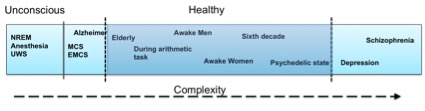
We still do not know exactly how brain complexity works but there have been several scientific studies that tackle the problem in various scenarios. Summarizing some research findings it seems that stroke patients, schizophrenia, and depression patients have higher LZ complexity on both a spontaneous and a cognitive task-related EEG activity compared to age-matched healthy controls (e.g., [1]). However, spontaneous EEG complexity seems to decrease during anesthesia, NREM sleep, as well as in Unresponsive Wakefulness Syndrome (UWS), Minimal Conscious State (MCS) or Emergence from MCS (EMCS) patients, and in Locked-in syndrome (LIS) patients [2]. Also, complexity seems to decrease in schizophrenia, depression and in healthy controls when the participants perform a mental arithmetic task compared to their resting state EEG [1]. Some of these findings are also supported by MEG (magnetoencephalography) studies, e.g., schizophrenia patients seem to have higher LZ complexity compared to healthy controls also in their MEG signals [3], and depressed patients seemed to have higher MEG pre-treatment complexity that decreases after 6 months of pharmacological treatment [4]. Although MEG and EEG refer to two distinct types of brain signals, it seems that their underlying complexity patterns follow a similar behavior. Other MEG studies have revealed decreased complexity in MEG signals in Alzheimer patients compared to age-matched healthy controls [5], increasing complexity until the sixth decade of life in healthy subjects, and decreased complexity after this age, as well as higher complexity in females compared to males [6]. A recent MEG study showed that the complexity is increased during a psychedelic state of consciousness induced using ketamine, LSD, and psilocybin compared to a placebo effect [7]. So, what is happening in the brain that gives way to some cases in which complexity increases whereas in other cases it decreases? Let’s explain some of the cases below.

Let’s begin with the decrease in complexity during the simple arithmetic task, compared to spontaneous EEG activity. Why does complexity decrease in this case? According to [1], a possible explanation is that the decrease in complexity may be due to an increase in synchronization during the mental activity, which typically reflects the state of internal concentration. Thus, the more concentrated, the better the brain is at being organized which results in lower complexity. Regarding schizophrenia and depression increases in complexity during the task and during the spontaneous activity compared to healthy controls, the same paper ([1]) suggests that this happens due to an increase in neuron participation in the information processing for both disorders. Thus, it seems that to perform the same task, schizophrenia and depressive patients require more neurons compared to healthy controls. In the same study it was found that schizophrenia patients had higher complexity compared to depressed ones, the latter of which was found to be closer to the healthy controls. This suggests that information processing in schizophrenia patients may require the participation of more neurons or more connections between them compared to both healthy controls and depressive patients. But does increased complexity always imply deficit? The answer is no.

As previously discussed, several studies have found increasing complexity with age in healthy subjects until the age of sixty and decreasing complexity later on, as well as increased complexity in females compared to males [6]. As reasoned in [8], these findings may be the result of capturing the continuous formation and maturation of the neuronal assemblies, and the development of cortico-cortical connections of neural assemblies with age, which starts decreasing after middle age. According to [6], this rationale coincides with the myelination of cortical white matter development with age, which is involved in the cortico-cortical connections. Specifically, the cortical white matter increases until it reaches a peak at around the fourth decade of life, and then decreases. This behavior has been verified by various brain imaging studies. This explanation doesn’t mean of course that only if there are changes in the white matter there will be changes in the complexity, but rather that changes in the white matter can provoke changes in the cortical complexity. So far there have been no observations on differences in the white matter between males and females, and it is still more difficult to explain the increased complexity observed in females compared to males.

Increased complexity was also found during a psychedelic state induced using ketamine, LSD, and psilocybin [7]. In this case, the increase in complexity seems related to richer, more expansive and diverse scenes compared to normal ones, according to the participants’ reports. The increase in complexity could be explained by an increase in neuron participation and higher connectivity across them due to the increase in the sensory information. Thus, the idea would be that since the environment is perceived as more enhanced and more diverse, more neuronal mechanisms would need to take place to perceive it. The authors of this paper relate their findings with bridging the gap between conscious content and conscious level, in the sense that increases in conscious level correspond to increases in various ranges of conscious content.

Now, let’s see what happens in the cases in which complexity decreases. As discussed previously, complexity decreases in dreaming, NREM, MCS, LIS, and anesthesia-induced stages [2]. The research carried out in this regard used a perturbation-driven protocol to trigger a significant response and measure this response through complexity. Among these stages, the estimated metric of complexity, namely the PCI (perturbation complexity index, based on LZc), behaved the same way depending on whether the loss of consciousness was due to a physiological process or due to a pharmacological intervention. Thus, NREM sleep stages, induced anesthesia, and UWS patients resulted in similar complexity values that were lower than the MCS/EMCS that was lower than the awake healthy controls. The complexity, as estimated in this case, measures both the information content and the integration of the output of the corticothalamic system, as explained by the authors.

So, what should the aim be: high or low brain complexity? Figure 1 presents the evolution of complexity with respect to various states, in an intuitive way. As with everything else in life, it seems that neither too much nor too little complexity in the brain can serve one right on well being, as can be seen from where the healthy part is lying on the complexity spectrum. There is still much room for understanding the whole complexity picture, as there are still missing relationships in the complexity spectrum, but don’t worry… We are working on that! If you are interested in the concept, you can also have a look at our H2020 Luminous project on studying, measuring and modifying consciousness. Keep an eye out for new findings resulting from our work! I hope this post helps you wrap your mind around the complex matter of complexity.

Figure 1. Intuitive description of the complexity spectrum

References:

[1]. Li, Yingjie, et al. “Abnormal EEG complexity in patients with schizophrenia and depression.” Clinical Neurophysiology 119.6 (2008): 1232-1241.

[2]. Casali, A. G., Gosseries, O., Rosanova, M., Boly, M., Sarasso, S., Casali, K. R., … & Massimini, M. (2013). A theoretically based index of consciousness independent of sensory processing and behavior. Science translational medicine, 5(198), 198ra105-198ra105.

[3]. Fernández, A., López-Ibor, M. I., Turrero, A., Santos, J. M., Morón, M. D., Hornero, R., … & López-Ibor, J. J. (2011). Lempel–Ziv complexity in schizophrenia: a MEG study. Clinical Neurophysiology, 122(11), 2227-2235.

[4]. Méndez, M. A., Zuluaga, P., Hornero, R., Gómez, C., Escudero, J., Rodríguez-Palancas, A., … & Fernández, A. (2012). Complexity analysis of spontaneous brain activity: effects of depression and antidepressant treatment. Journal of Psychopharmacology, 26(5), 636-643.

[5]. Gómez, C., & Hornero, R. (2010). Entropy and complexity analyses in Alzheimer’s Disease: An MEG study. The open biomedical engineering journal, 4, 223.

[6]. Fernández, A., Zuluaga, P., Abásolo, D., Gómez, C., Serra, A., Méndez, M. A., & Hornero, R. (2012). Brain oscillatory complexity across the life span. Clinical Neurophysiology, 123(11), 2154-2162.

[7]. Schartner, M. M., Carhart-Harris, R. L., Barrett, A. B., Seth, A. K., & Muthukumaraswamy, S. D. (2017). Increased spontaneous MEG signal diversity for psychoactive doses of ketamine, LSD and psilocybin. Scientific Reports, 7.

[8]. Anokhin, A. P., Birbaumer, N., Lutzenberger, W., Nikolaev, A., & Vogel, F. (1996). Age increases brain complexity. Electroencephalography and clinical Neurophysiology, 99(1), 63-68.

Attention Deficit Hyperactivity Disorder (ADHD) is a neurodevelopmental disorder characterized by problems in paying attention[1] (the incapacity of attending with a necessary degree of constancy to any object), hyperkinetic activity (remarkable motor activity which appears urgent) and a lack of controlled behavior (unstable mood, fits of rage, tendency to aggressively or excitability) that interferes with functioning or normal development [1,2].

This disorder was formally conceptualized as a pathological disorder at the US in 2000 (on the DSM-IV-TR[2]). Within the European clinical practice, ADHD was first diagnosed with precise metrics and clinical scales in 1993 as defined within the ICD-10 classification list. Before that, ADHD symptoms were diagnosed as hyperkinetic disorders or attention deficit disorder (ADD) although its treatment through medication and the consideration of ADHD as a psychiatric disorder only became significant in the 1970s [6].

‘When any object of external sense, or of thought, occupies the mind in such a degree that a person does not receive a clear perception from any other one, he is said to attend to it’

Alexander Crichton, 1798

Current clinical diagnostic criteria involve a qualitative evaluation of impaired attention levels, hyperactivity and lack of controlled behavior (involving deshinibition, recklessness or impulsivity) based on the criteria described in DSM/ICD medical classifications list. As the two guidelines are slightly different, the prevalence of the disease will vary according to which criterion is applied. In particular, DSM-IV criteria diagnoses 5-7% of children [4], while ICD-10 shows a 1-2% diagnose rate in children [5].

Additionally, as both hyperactivity and inattention also arise as a symptom of anxiety or depressive disorders in children [9], both clinical diagnose guides require that ADHD is only diagnosed when the symptoms are not better explained by any other disorder. As to increase specificity of the diagnose and phenotype that ADHD describes, three subtypes of ADHD are described in both clinical manual for diagnosis (DSM and ICT):

• ADHD-I: predominantly inattentive type
• ADHD-H: predominantly hyperactive/impulsive subtype
• ADHD-C: combined type

However, the clinical classification of ADHD still lacks a neurophysiological counterpart, and in fact, different ADHD subtypes have been proposed based on electrophysiological signals (see [11] or [12] for more details).

With this complexity in mind, current qualitative evaluation of ADHD results in a diagnostic accuracy of 61% [13]. Such accuracy has been recently improved by clinical decision support systems (DSS) that involve the analysis of resting-state EEG to the 88% (see [13], the TBR test), although it’s clinical relevance in separating different subtypes remains under discussion.

Despite the complications in diagnosis, ADHD is described as a disorder that impairs the appropriate development and functioning of the patient. For this reason, it’s early and an accurate diagnose of ADHD becomes crucial as to treat and ensure an appropriate development and functioning of the patient.

In terms of treatment, current therapies for ADHD are varied and involve combination of counseling, medication and lifestyle changes [2]. Medications for ADHD are mostly based on stimulants (i.e amphetamine, methylphenidate, etc) that block the dopamine and nor-adrenaline pathways, drugs that in normal children/adults is reported to enhance focal attention and general performance-enhancement [6]. Note however that, to this date, there is no knowledge on which medication improves symptoms with lower side effects and they are currently applied as ‘trial and error’ for each diagnosed children [7]. Additionally, a recent longitudinal study report that stimulant medication; behavior therapy or multimodal treatments in ADHD have limited long-term beneficial effects [8].

This overall situation opens the question of whether further understanding of the neurological aspects of the disease is needed, opening the door to the development of quantifiable biologically-driven markers of ADHD.

1. Cormier E. Attention Deficit/Hyperactivity Disorder: A Review and Update. J Pediatr Nurs. 2008;23: 345–357. doi:10.1016/j.pedn.2008.01.003
2. Attention Deficit Hyperactivity Disorder. Natl Inst Ment Heal. 2016;
3. FORD T, GOODMAN R, MELTZER H. The British Child and Adolescent Mental Health Survey 1999: The Prevalence of DSM-IV Disorders. J Am Acad Child Adolesc Psychiatry. Elsevier; 2003;42: 1203–1211. doi:10.1097/00004583-200310000-00011
4. Willcutt EG. The Prevalence of DSM-IV Attention-Deficit/Hyperactivity Disorder: A Meta-Analytic Review. Neurotherapeutics. 2012;9: 490–499. doi:10.1007/s13311-012-0135-8
5. Cowen P, Harrison P, Burns T. Shorter Oxford textbook of psychiatry. Oxford University Press; 2012.
6. Lange KW, Reichl S, Lange KM, Tucha L, Tucha O. The history of attention deficit hyperactivity disorder. ADHD Atten Deficit Hyperact Disord. 2010;2: 241–255. doi:10.1007/s12402-010-0045-8
7. McDonagh M, Peterson K, Thakurta S, Low A. Pharmacologic Treatments for Attention Deficit Hyperactivity Disorder. Oregon Heal Sci Univ. 2011; Available: https://www.ncbi.nlm.nih.gov/books/NBK84419/pdf/Bookshelf_NBK84419.pdf
8. Molina BSG, Hinshaw SP, Swanson JM, Arnold LE, Vitiello B, Jensen PS, et al. The MTA at 8 Years: Prospective Follow-up of Children Treated for Combined-Type ADHD in a Multisite Study. J Am Acad Child Adolesc Psychiatry. 2009;48: 484–500. doi:10.1097/CHI.0b013e31819c23d0
9. WHO. The ICD-10 Classification of Mental and Behavioural Disorders. IACAPAP E-textb child Adolesc Ment Heal. 2013;55: 135–139. doi:10.4103/0019
10. Clarke AR, Barry RJ, Dupuy FE, Heckel LD, McCarthy R, Selikowitz M, et al. Behavioural differences between EEG-defined subgroups of children with Attention-Deficit/Hyperactivity Disorder. Clin Neurophysiol. International Federation of Clinical Neurophysiology; 2011;122: 1333–1341. doi:10.1016/j.clinph.2010.12.038
11. Ogrim G, Kropotov J, Hestad K. The quantitative EEG theta/beta ratio in attention deficit/hyperactivity disorder and normal controls: Sensitivity, specificity, and behavioral correlates. Psychiatry Res. Elsevier Ltd; 2012;198: 482–488. doi:10.1016/j.psychres.2011.12.041
12. Arns M, Gunkelman J, Breteler M, Spronk D. EEG phenotypes predict treatment outcome to stimulants in children with ADHD. J Integr Neurosci. 2008;7: 421–438. doi:10.1142/S0219635208001897
13. Snyder SM, Rugino TA, Hornig M, Stein MA. Integration of an EEG biomarker with a clinician’s ADHD evaluation. Brain Behav. 2015;5: 1–17. doi:10.1002/brb3.330
14. NEBA HEALTH L. De novo classification Request for Neuropsychiatric EEG-based assessment AID for ADHD (NEBA) system. FDA. 2011;

[1] According to [6], altered behavior in ADHD is clearly represented in ‘The story of fidgety Phillip’, drawn by the famous psychiatrist Heinrich Hoffman.

[2] DSM is the acronym for the Diagnostic and Statistical Manual of Mental Disorders, a manual published by the American Psychiatric Association to offer standardized criteria for the classification of mental disorders used worldwide. The EU equivalent is the ICD- International Statistical Classification of Diseases and Related Health Problems as published by the WHO.

Heart monitoring is becoming increasingly popular with the availability of health monitoring wristbands. Most of these units have built-in microprocessors that analyze the recorded signals (*1) to determine the heart rate – the frequency of the cardiac cycle (beats per minute). But, besides the heart rate, what can we learn from our heart?

The cardiac cycle is controlled through electrical impulses (action potentials), induced by pacemaker cells within the sinoatrial node (SA). Their impulse creates a generalized contraction of the muscle cells, which spreads through the heart. As the electrical impulse travels from the pacemaker cells (located in the top of the hart) from the top of the heart to the bottom, it causes the heart to contract and pump blood through heart cavities, whose combined contraction make up the heartbeat. The rhythm of the pacemaker cells within the SA directly controls the heart rate, which at rest is between 60-100 beats per minute [1].

Determining the cardiac cycle and its dynamics can be done a continuous monitoring of the heart activity, a process can be measured through the analysis of blood flow or by analyzing the electrical activity of the heart muscles*2. The latter is known as electrocardiogram or ECG/EKG (see Figure 1 for an example), and can be done by electrical monitoring sensors like Enobio or Starstim by NE. EKG sensors can be then used to monitor the spread of electrical activity through the heart, a pattern that reflects the activity of the different muscles of the heart, see inlet of Figure 1 for a single cardiac cycle. The relation between the EKG and the underlying electrical activity of a cell is rooted in electromagnetism: a depolarization of the cells towards the positive electrode produces a positive deflection in the EKG. Or in other words, the P wave reflects the depolarization of the upper part of the heart initiated by the SA node; QRS reflects the depolarization of the lower part of the heart and T corresponds to the repolarization that starts at the bottom of the heart. Additionally, in an EKG, different electrodes record electrical activity from different parts of the heart and therefore, reflect activation of different muscles (Figure 1). So, once we can determine the cardiac cycle, what can we learn from them? Below you will find a set of metrics that can be extracted from the cardiac cycle as to analyze the properties of the heartbeat.

• R-R interval: defined as the interval between two heartbeats, which reflects the completion of a cardiac cycle. This metric is actually used to assess the heart rate, which in turn can reflect the action of the CNS (see this post for interesting insights on the R-R interval).
• Heart rate variability (HRV): reflects the variation in the time interval between heartbeats (RR variability) or how regular is the interval between beats. HRV in healthy subjects is related to emotional arousal –
• Cardiac efficiency, a concept proposed by Bing et al in 1949 [2], aims to measure how well the energy used by the heart is transformed into actual work. The efficiency of a healthy heart is approximately 20-25% and reductions in this metric are an important prognostic for patients that may undergo cardiac arrest [3]. In wearable technology, this can be translated into a simple metrics of ‘steps per minute/beats per minute’ and although it’s clinical estimation is more complex, it has been propose to serve as a sufficient approximation [3].

Figure 1 Channel V2 of an electrocardiogram (ECG or EKG) for different subjects (S1 to S3) and the same subject that is exposed to two different medications (S3 and S3’). At the inset, the nomenclature that specifies different parts of the cardiac cycle (for an animated cardiac cycle image, see here)

Importantly, cardiac cycle and its metrics are regulated by physical exercise through the secretion of acetylcholine (that directly signals the SA node). But is not only exercise that modulates the signaling of acetylcholine. Sleep-wake cycle, thermoregulation or meals affect the heart rate through the SA signaling. Stress, sadness or happiness also alters the heart signaling system. Heartbeat does not only change with internally generated emotions but its variability also changes depending on the mood of the music that you are hearing [5]. In fact, several machine-learning algorithms are being developed as emotion recognition systems, which would allow for the clear differentiation of several emotions based on heart rate metrics (see [4] for instance).

Despite the variety of metrics that can be obtained from heartbeat trackers, its information is barely included in the medical system by health professionals. And the limitation relies in that the vast majorities of commercially available wearables have not been tested in clinical settings and thus, lack approval by the regulatory agencies as medical devices. What would the future bring us? Like mobile phones, wearables enable the user to become autonomous – will we become autonomous towards our health?

[1] Gordan, Richard, Judith K. Gwathmey, and Lai-Hua Xie. “Autonomic and endocrine control of cardiovascular function.” World journal of cardiology 7.4 (2015): 204.

[2] Bing RJ, Hammond M, Handelsman JC, et al. The measurement of coronary blood flow, oxygen consumption and efficiency of the left ventricle in man. Am Heart J. 1949;38:1–24

[3] Visser, Frans. “Measuring cardiac efficiency: is it clinically useful?.” Am Heart J38 (1949): 1-24.

[4] Yu, Sung-Nien; Chen Shu-Feng; Emotion state identification based on heart rate variability and genetic algorithms. Conf. Proc IEE Eng Med Biol Soc. (2015) Aug:538-41.

[5] Nakahara, Hidehiro, et al. “Emotion‐related Changes in Heart Rate and Its Variability during Performance and Perception of Music.” Annals of the New York Academy of Sciences 1169.1 (2009): 359-362.

*1: Newest devices are optical sensors, generating a signal that is also known as a photoplethysmogram (PPG) – LED lights emit light that it is naturally absorbed by our skin and blood. A photoreceptor reads out the amount of absorbed light – which is larger when a heartbeat pushes all the blood through the sensor.

*2: Other sensors that can be use to monitor heart include pulse oximetry (measure oxygen saturation) or seismocardiogram (records body vibrations induced by heart beat).

Artificial Intelligence (AI) has been part of our imaginations and simmering in research labs since a group of computer scientists rallied around this topic at the Dartmouth Conference in 1956. They would give birth to the field of AI.

In the decades since, AI has exploded, especially since 2015. Much of that has to do with the wide availability of GPUs. They make parallel processing ever faster, cheaper, and more powerful. It also has to do with the simultaneous increase in storage capacity and a flood of data of every stripe. (That whole Big Data movement) – images, text, transactions, mapping data, etc.

The two main milestones in AI that have made significant advancements in the field are Machine Learning and Deep Learning.

Machine Learning is the practice of using algorithms to parse data, learn from it, and then make a determination or prediction about something in the world. This is at its most basic. Rather than hand-coding software routines with a specific set of instructions to accomplish a particular task, the machine is “trained”. How? By using large amounts of data and algorithms that give it the ability to learn how to perform the task.

Deep Learning enables many practical applications of Machine Learning and by extension the overall field of AI. Deep Learning breaks down tasks in ways that make all kinds of machine assists seem possible, even likely. Driverless cars, better preventive health care, even better movie recommendations, are all here today or on the horizon. AI is the present and the future. With Deep Learning’s help, AI could make that science fiction state a reality.

How can we apply AI, Machine Learning or Deep Learning to EEG data? There is evidence that EEG characteristics can be used as an indication (a biomarker) of some diseases. For example, in a project funded by The Michael J. Fox Foundation, our findings indicate that there are significant differences in the EEG data of different RBD patients compared to healthy populations. More specifically, RBD subjects as a group had larger power in the frontal EEG electrodes than healthy subjects. Again taken as a group. Therefore, there is statistical significance in the difference between one group and the other. However, if we want to use this as a means for diagnosis, we need to take into account that diagnostic decisions are made on individuals, not on groups. For this to happen we need a decision system. We would input the data of a particular individual subject. Then we would get an answer on whether this individual is likely to develop, for instance, a neurodegenerative disease. Here is where Machine Learning and Deep Learning come into play.

We designed an early diagnostic system based on Echo State Networks (ESN) that takes specific features of EEG data as an input. This input can predict if the subject is likely to develop Parkinson’s Disease (PD) 10-15 years before developing any symptoms. We obtained excellent results by predicting individual PD development with 85% accuracy [1]. More recently, other deep learning techniques allowed us to achieve a similar performance while reducing the computational cost and avoiding the need for feature selection [2]. This would allow implementing preventive treatments before the disease actually develops and it is too late for treatment.

In the near future, we envision these techniques to enable early diagnosis systems for the detection of neurodegenerative diseases. We can also use them to show signature patterns in physiological data. This can range from spine injuries to heart disease or cancer. This could even change how we treat early diagnosis.

Here at Neuroelectrics, we strive to move the marker to make technology that can effect positive change in the future. Want to know more about Neuroelectrics’ EEG products? Click Here

[1] Ruffini G, Ibáñez D, Castellano M, Dunne S, Soria-Frisch A. EEG-driven RNN classification for prognosis of neurodegeneration in at-risk patients. ICANN 2016 2016;

[2]Giulio Ruffini, David Ibanez Soria, Laura Dubreuil, Jean-Francois Gagnon, Aureli Soria-Frisch. Deep learning using EEG spectrograms for prognosis in idiopathic rapid eye movement behavior disorder (RBD). bioRxiv 240267; DOI: https://doi.org/10.1101/240267 (2018)

The post How can we apply AI, Machine Learning or Deep Learning to EEG? appeared first on Blog Neuroelectrics.

Transcranial current stimulation (tCS) seems to be a powerful tool to make the link between brain function and disease. This has been demonstrated in current research. However, we have yet to fully understand the underlying neurobiological mechanisms of tCS. The goal of combining tCS with neurophysiological and neuroimaging tools is twofold: a) these techniques can provide information about when, where, and how to stimulate the brain and help to improve precision and accuracy of stimulation, and b) these techniques provide information about the neural changes induced by tCS, helping to better understand its neurobiological mechanisms.

Why would one like to combine tCS with various neuroimaging and electrophysiological tools? The answer is pretty simple: the various existing techniques provide complementary information, they somehow answer the same question but through different pathways, shedding light on different underlying mechanisms of brain function.

They all associate specific temporal and spatial brain patterns with certain cognitive functions, in a way that depends on their intrinsic properties. Before going through the technological differences of these tools, let’s see what do they measure and how they are related to tCS.

Neural activity generates electrical potentials in the brain that can be measured by electroencephalography (EEG). These potentials give rise to a magnetic field that can be measured by magnetoencephalography (MEG). EEG and MEG belong to the category of electrophysiological tools and measure the direct output of neurons, which is their electromagnetic field. These generated electrical potentials and consequent magnetic field result in an increase in glucose and oxygen demands that leads to an increase in the local hemodynamic response. This process is known as neural metabolism and can be captured by neuroimaging tools, such as functional Magnetic Resonance Imaging (fMRI) and Near-Infrared Spectroscopy (NIRS). The role of tCS in this process is that it modulates the level and/or timing of excitatory or inhibitory activity patterns, which affect cortical excitability (measured by electrophysiology) that in its turn affects the local hemodynamic response (measured by neuroimaging).

To briefly compare these tools, EEG and MEG are known for their excellent temporal resolution, which is provided in milliseconds compared to fMRI that has resolution in seconds. EEG is cheap, easy to set up and carry, you can use it even at home, and you can measure using the same device as tCS (e.g., our Starstim device). The strong point of MEG over EEG is that it allows for assessing brain activity even underneath the stimulation electrodes, due to the fact that it does not suffer from the volume conduction phenomenon present in EEG. However, its drawback with respect to EEG is that it is more expensive and is not portable. Neuroimaging tools outperform electrophysiology tools in terms of spatial resolution. For instance, fMRI provides spatial resolution in 2-4mm whereas EEG in cm. Due to its good spatial resolution, fMRI reveals stimulation effects on interconnected brain regions, either in remote or in neighboring regions. If you are interested in good spatial and temporal information at the same time, NIRS is a good compromise between temporal (around 100msec) and spatial resolution (30mm), and compared to fMRI is cheaper and portable.

If you are new to tCS research, and you are wondering on how to start, I would advise you to choose the electrophysiology/neuroimaging method based on the differences presented above, start from an already known problem, and see how tcs modifies it. For example, in (Helfrich et. al., 2015), the authors knew a-priori that the cross-frequency coupling (CFC) between alpha and gamma EEG bands seems to be responsible for visual processing organization, attentional control, and short-term visual memory. Entraining with tACS (transcranial alternate current stimulation) the alpha (10Hz) and gamma (40Hz) EEG bands, they found significant differences between tACS and sham in the CFC of alpha and gamma, showing evidence for modulation of CFC with tACS.

In a tDCS (transcranial direct current stimulation) combined with MEG study (Hanley et. al., 2015), starting from the known relationship between beta band and motor activity, as well as between gamma band and visual activity, the authors revealed significant reduction both in motor beta and in visual gamma power with tDCS during a visuomotor task compared to sham. This result provides evidence for modulation of MEG features with tCS. Similarly with tCS and fMRI, knowing that BOLD (Blood Oxygen Level Dependent activity) changes in the occipital cortex are related to visual processing, the authors (Vosskuhl et. al., 2015) found reduced BOLD signal changes in the occipital cortex with IAF (Individual Alpha Frequency) –tACS stimulation during a visual vigilance task. Finally, in a NIRS-tDCS study (Ehlis et. al., 2015), starting from the fact that a word fluency task has as consequence extensive activation of the frontal cortex, the authors revealed significant changes in oxygenated hemoglobin by stimulating the prefrontal cortex during verbal word fluency, indicating that tCS has measurable effects in the NIRS signal.

Hence, when we want to measure tCS effects on neuroimaging and electrophysiology it’s important to select the appropriate metrics to capture brain changes, as in the above examples. However, let’s not forget that we are still at the beginning of the tCS era meaning that there is still limited knowledge on the underlying mechanisms of tCS and on how these mechanisms can be measured. Thus, methodological studies to determine appropriate and relevant metrics are necessary.

References:

Helfrich, R.F., et al., Different couplingmodes mediate cortical cross-frequency interactions, NeuroImage (2015), http://dx.doi.org/10.1016/j.neuroimage.2015.11.035

Hanley, C.J., et al., Transcranial modulation of brain oscillatory responses: A concurrent tDCS–MEG investigation, NeuroImage (2015), http://dx.doi.org/10.1016/j.neuroimage.2015.12.021

Vosskuhl, et. al., BOLD signal effects of transcranial Alternating Current Stimulation (tACS) in the alpha range: A concurrent tACS-fMRI study, NeuroImage (2015), doi:10.1016/j.neuroimage.2015.10.003

Ehlis, A.-C., et al., Task-dependent and polarity-specific effects of prefrontal transcranial direct current stimulation on cortical activation during word fluency, NeuroImage (2016), http://dx.doi.org/10.1016/j.neuroimage.2015.12.047

The post Monitoring effects of Transcranial Current Stimulation with EEG, fMRI, MEG, NIRS. appeared first on Blog Neuroelectrics.

Clustering methods are in charge of grouping sets of data objects with the aim of finding relationships within the objects that compose the data. Such a process allows the data scientist to find similarities within the data, draw inferences, find hidden patterns and also to reconstruct a possibly underlying data structure. For example the relative connectivity within the data. In machine learning (ML) literature, clustering is one of the methods that is normally used in unsupervised learning with the aim of learning the underlying hidden structures of the data and its categorization.

Therefore, there is great interest in carrying out a clustering task in an exploratory analysis to find new insights. We know that there are different clustering methods and each method has been proven to provide accurate clustering results in different fields. However, how can we choose the best clustering algorithm for our data analysis task? and how can we assess the best number of clusters ?

Having these two questions in mind I will briefly summarize some of the most common clustering methods that have shown relevant applicability. Additionally, I will comment on the criteria that should be taken into account when performing clustering and comment on the most well-known methods for accessing how good your clustering is.

Clustering algorithms

To begin with it is good to bear in mind that there are different types of clustering outputs performed by the clustering methods. These types of clustering are known as hard and soft clustering. The difference between these two methods of clustering is that in soft clustering one object can belong to more than one cluster, whereas in hard clustering an object belong to only one cluster. Additionally, there are different ways to approach the clustering problem. While some methods tend to find the possible underlying distributions of the data or the density of the data, other methods focus on the distance between the neighboring points and their connectivity.

The list of algorithms to carry out clustering is quite extensive. Thus, I have only picked up some of them to comment in this article bearing in mind the different ways they perform the clustering and therefore the different situations in which they can be very useful.

K-means it will be hard to find a clustering article with no mention to the well-known K-means algorithm. K-means is a hard clustering algorithms (there also implementations for soft clustering) that assign objects to an initial k number of clusters, then initial clusters are iteratively re-organized by assigning each entry object to its closest cluster (centroid) and re-calculating cluster centroids until no further changes take place. The optimizing criterion in the clustering process is the sum-of-squared-error E between the objects in the clusters and their respective cluster centroids. This method is commonly used as a first approach for clustering, has the particularity that tend to find cloud of clusters within a distance range to its centroid. As a drawback it might be conditioned by the initial position of its centroids (initialization problem) and tend to not work well with data that lies in a convex geometric shape. In exploratory analysis, K-means can also be used to detect possible outliers in the data. Below in figure 1 you can find an example of how K-means learn the positions of the centroids. (This example has been borrowed from r-bloggers.com).

Fig 1. K-means centroids learning process

Hierarchical clustering is a different type of clustering that is based on the concept of proximity. The algorithm build nestles clusters by merging or splitting them successively. This hierarchy of clusters is represented with a tree diagram called a dendrogram. The linkage criteria determines the distance between sets of objects as a function of the pairwise distances between the objects. Therefore, choosing different distance criteria can lead to different clustering outputs. This method finds hard clusters and allows you to find cluster object connectivity properties. As a drawback hierarchical clustering methods are not very robust towards outliers, which will either show up as additional clusters or even cause other clusters to merge. In exploratory analysis, hierarchical clustering can be used not only for clustering but also to find underlying connectivity properties. In contrast to K-means it works well with convex geometric data shapes. It is an interesting clustering method for image segmentation in image processing. Below in figure 2 you can find an example of a dendrogram in hierarchical clustering.

Fig 2. Dendrogram example in hierarchical clustering

Gaussian Mixture Models (GMM) is another type of clustering based on distribution models where cluster objects are very likely to belong to the same distribution. Thus, GMM is a probabilistic model that represents the presence of sub populations within an overall population, without requiring that an observed data set should identify the sub-population to which an individual observation belongs. Formally a GMM corresponds to the mixture distribution that represents the probability distribution of observations in the overall population. GMM is used to make statistical inferences about the properties of the sub-populations given only observations on the pooled population, without sub-population identity information. This is a soft clustering method that in many scenarios outperforms k-means and works very well for data with implicit Gaussian distributions. As a drawback this distribution based clustering tend to suffer from the over-fitting problem, when not initialized with a fixed number of Gaussian distributions (a given k clusters). In exploratory analysis, GMM could be a very interesting clustering method specially when the data might follow a combination of Gaussian distributions. Below in figure 3 you can find an example of an example of GMM using different types of Gaussian distributions.

​ Fig 3. Gaussian Mixture Example (scikit-learn library)

Other very interesting clustering algorithms not mentioned in this post are:

• Spectral clustering
• Density-based spatial clustering (DBSCAN)
• Self organised maps (SOM)

Validity criteria

Validity criteria methods are a way to assess how good our clustering is. Put it in another way, we know our algorithm will always throw back to us a given clustering. So, in a purely exploratory analysis scenario these are the means by which we make sense of our clustering. It helps to avoid finding patterns in noise, to compare clustering algorithms and to compare two sets of clusters.

The two types of validity criteria that are mostly used are: external and internal index.

External Index

External indexes are used to assess if a given clustering correlates to previous information about categories of the data. This means, that there is a previous knowledge about present categories in the data and therefore the goal of the clustering is to verify if our clustering output correlates to these categories.

Put it in another way, the external indexes can be used to:

• Measure the extent to which cluster labels match externally supplied class categories.
• Compare the results of a cluster analysis to externally known results.

Known external index methods: Purity index, F-measure and other measures borrowed from supervised learning to measure accuracy.

Internal Index

In a pure blind exploratory data analysis, internal indexes are used to evaluate the “goodness” of the resulting clusters and it also tries to determine the ‘correct’ number of clusters that should be used by some of the clustering methods for the K number of desired clusters.

A good clustering algorithm should generate clusters with high intra-cluster homogeneity, good inter-cluster separation and high connectedness between neighboring data objects. To achieve this aim, internal index address to measure:

• The cluster cohesion (how close the points belonging to the same cluster are)
• The cluster separation (how distinct or well separated a cluster is from others)

• The goodness of a clustering structure without respect to external information.
• How well the results of a cluster analysis fit the data without reference to external information

Known internal index methods: Sum of square errors, Silhouette coefficient, Bayesian information criteria (BIC), Explained variance (Elbow method).

Summary

Different methods for clustering have been presented together with the validity criteria to be taken into account when assessing the quality of the clustering. So how can we choose the best clustering algorithm for our data analysis task? How can we assess the best number of clusters ?

Well, at this point it comes to the data someone might be dealing with. Each clustering algorithm will produce different clustering results which might be very similar depending on the underlying data structure or could be totally different. So having a clear idea of the desired goals of the clustering analysis and the sources of the data someone is dealing with, would definitely help to better chose the right algorithm and its right validity measure to assess the right number of clusters.

Last but not least, data visualization is a very powerful tool to assess how close you are to your clustering goals and to know the kind of data you might be dealing with. However, choosing the right way to visualize your data in the case of having to perform dimensionality reduction will play a mayor roll when interpreting your data. In further post, i will address other clustering methods and some of the dimensionality reduction techniques.

The post Clustering Methods in Exploratory Analysis appeared first on Blog Neuroelectrics.

Have you ever imagined how many sensors, signal processing and subtasks it takes for the body to process and execute a success command?

The recent paper by Crea et al (Scientific Reports 2018) represents an exciting step towards the development of practical brain-computer interfaces (BCI). In this case, the development is designed for patients with large deficits in arm and finger control that affect daily activities such as drinking or eating – which we usually take for granted.  Such impairments arise from spinal cord injuries or stroke, for example, and have a very large impact on quality of life. 

The BCI in this paper is a complex system that combines a whole-arm exoskeleton designed to integrate EEG and EOG (electrical signals from the brain and eye movements) for reaching and grasping control. The main challenge is to individualize the system while making it user-friendly, safe and effective. 

As the authors point out, recent work with invasive measurements (e.g.,  see this and this) have delivered impressive results. Implantation, however, has its risks and morbidity. The authors in this paper (led by Surjo Soekadar) have demonstrated in previous work (with our admired advisor Niels Birbaumer) the feasibility of asynchronous EEG/EOG BCIs for grasping. By this, we mean interfaces that can be used at any time, without synchronization to timing cues (which if present facilitate enormously the algorithmic end of things, although reducing significantly user experience).  

Crea et al. go beyond that one in two aspects. First, they extend the interface. In the authors’ words,  “In contrast to a simple grasping task, operating a whole-arm exoskeleton, for example, to drink, involves a series of sub-tasks such as reaching, grasping and lifting.” This extension translates into a much bigger space of possible actions, with a large number of degrees of freedom. The requirements for information transfer bandwidth rapidly explode. To handle this, robotics comes to the rescue in the form of a vision-guided autonomous system. Similar processes occur in the brain, where “automatized” tasks are not consciously controlled.  In other words, the system represents a fusion of human and machine intelligence connected by EEG and EOG signals. Robot and human collaborate for the task of reaching and grasping a glass of water, drinking, and placing it back on the table.  The human is on top of the command chain, initiating the reaching action (via EOG signals) and grasping (via EEG) – see this figure below.

As for EEG/EOG, the authors use Neuroelectrics’ Enobio wireless system using 6 solid gel electrodes.  Using BCI2000, these signals were translated into commands for shared control of the exoskeleton with the robotic vision-guided system. The latter was used to track and reach the object to be grasped. The overall system is quite complex, involving IR cameras, Enobio, exoskeleton components (hand-wrist and shoulder elbow) and a visual interface. Most of the communications across sub-systems was mediated by TCP/IP (e.g., Enobio’s software, NIC, can stream EEG data continuously over a network).   

The end result will remind sci-fi fans of the concept of a  cyborg, or more precisely of a Lobster (made not by using internal implants, but by using a smart external shell as the one worn by Iron-Man).  It is the fascinating meld of human and artificial intelligence with robotics that makes this and similar developments exciting, as they bypass the bandwidth limitations of BCIs through shared control with an exocortex. As all the technology elements in such systems evolve (sensors, signal processing, AI, robotics) and coalesce, their impact will be enormous and probably spill over to consumer applications. After all, all you may really want is to drink that glass of water, not worry about the million details that actually go into realizing that stupendous feat. 

The post Practical BCI Application: the feasibility of asynchronous EEG/EOG BCIs for grasping appeared first on Blog Neuroelectrics.

Let’s face it: frogs are not the most glamorous of animals…However, we owe a great deal to them! In 1780, Luigi Galvani found out that muscles of frog’s legs would twitch if in contact with electrical stimuli.

Today we know that this is due to one remarkable property of biological tissues: the fact that they can actively respond to electric signals. This is enabled by the presence of ions in the extracellular and intracellular compartments, and by the fact that cells in our body such as neurons and muscular cells have ion channels in their membranes that can control the flow of ions through it. The latter allow these cells to generate, propagate and transmit electrical oscillations of the membrane known as action potentials. Action potentials are the signals our brain uses to communicate…and compute! The electrical nature of these phenomena allows us to measure the electrical activity of certain organs with devices placed in contact with the skin, just as one would do to measure the voltage difference across a resistor in a high-school physics experiment!

Biosignal recording techniques like EEG and ECG take advantage of that. More intriguingly, we can use external current sources to alter the “normal” behavior of these cells. The latter generate an electric field (E-field) in the tissues which will affect the membrane potential of excitable cells. This is the case of non-invasive brain stimulation techniques such as transcranial current stimulation (tCS).

Figure 1: From left to right: electrostatic potential in the scalp due to models of neuronal activity placed on the brain surface of the model (in ); component of the electric field normal to the cortical surface of the brain (in ), due to current injection via the electrodes represented in the image.

But what is this E-field we have been talking about so much? The E-field is a vector, i.e., a mathematical entity that has, in each point in space, a direction and a magnitude (in Volts per meter). In conductive materials (like the ones in our heads), it drives an electric current: the E-field exerts a force on charged ions establishing a current. The E-field generated during tCS is thought to interact mostly with pyramidal cells in the cortex. According to cable theory^[1], which deals with the interaction between the E-field along a neuron and the changes in membrane potential it produces, an E-field directed along the pyramidal neuron and directed towards its soma will lead to an increase in soma excitability. The opposite happens when the E-field points from the soma to the apical dendrite. The fact that pyramidal cells tend to align perpendicularly to the cortical surface, suggests that the component of the E-field along this direction (En) is the most important one in predicting the effects of tCS^[2].

The E-field established in the brain during tCS depends on multiple factors: the geometry of the electrodes and the currents injected through them, the geometry of the head and the electrical properties of the tissues (like the electrical conductivity, i.e., a measure of how well a tissue conducts electric current)^[3]. The physics equations that allow us to calculate the E-field in the head, assuming we have knowledge about the previously listed parameters, are well studied and have been known for years from electromagnetism^[4]. However, only recently has it become possible to numerical solve these equations in a manner of hours, due to the available powerful computational resources!

The creation of a head model suitable for E-field calculations is usually based on MRI structural images. The latter are segmented into the different tissues comprising it. Usually models include scalp, skull (in some cases this is segmented into compact and spongy bone), cerebrospinal fluid (CSF), grey-matter (GM) and white-matter (WM). 3D surfaces of these tissues are then calculated based on the segmented masks. At this stage electrode models are also represented on the surface of the scalp.

The finite element (FE) method is normally used to numerically solve the equations and calculate the E-field in the head. In this method, the geometry of the head is discretized into simpler geometric shapes (finite elements). This geometric discretization is called the finite element mesh. A full explanation of the FE method is beyond the scope of this blog, but a (very) mathematically inclined reader can read more details in [5]. The FE method allows for the efficient and accurate calculation of an approximation to the E-field in each vertex of the FE mesh (nodes of the mesh).

Figure 2: Finite element head model depicting the E-field distribution in the brain. The color-scale indicates the normal component of the E-field (in V/m). Positive/negative values indicate an E-field directed into/out of the cortical surface. This E-field distribution was calculated for 35 cm² sponge electrodes located over the motor cortex (anode) and contralateral supra orbital area (cathode). The finite element mesh is shown over the right hemisphere.

After all this work, the brave researcher that has successfully created a head model is rewarded with a powerful tool that can, for example, be used as a complementary analysis to the results of an experiment using a specific montage to stimulate a group of subjects. These models can be created on a subject by subject basis, thus allowing for analysis of average En-field values in some regions of interest in the brain. A more interesting approach is to use these models during experimental design, to determine the montage that better targets a specific region (or a network of regions) in the brain^[6]. In NE’s Stimweaver implementation of this montage optimization the target is defined based on the type of desired effect (increase in excitability, decrease in excitability or no-change) and on the weight with which that effect should be enforced during the optimization. The algorithm^[2] then determines the optimized montage constrained by maximum number of electrodes, maximum total injected current and maximum current per electrodes.

Figure 3: Example of optimization for a complex cortical network. From left to write En-field in the GM surface (V/m); target En-map (red areas to excite, blue areas to inhibit); weight map.

In the eternal words of George Box, “(…) all models are wrong (…)” since all models make assumptions and simplifications of reality. However, we can ask ourselves: “Is the model illuminating and useful?”. The type of head models we have described in this blog entry have proven (and continue to do so) their usefulness in analyzing the E-field distribution in commonly used montages and in planning experiments. If you can look past an admittedly steep (at first) learning curve, you will be rewarded with a powerful tool that can really help your experiment reach the next level in terms of results…In any case our team at NE is always available to help you create these models and take full advantage of them!

Useful resources:

NIC software: Did you know you can use NIC to visualize the E-field distribution in any montage with PiStim electrodes? And you can do it in two available head models (one male and one female). We are always updating NIC so stay tuned for more features!

Stimweaver service: We perform optimization of montages in a standard head model with a target map that you can create here! We can also map more complex target maps to this subject or run optimizations based on personalized head models. For more information contact us.

References:

[1] Roth BJ. Mechanisms for Electrical-Stimulation of Excitable Tissue. Critical reviews in biomedical engineering. 1994;22(3-4):253-305.

[2] Ruffini G, Fox MD, Ripolles O, Miranda PC, Pascual-Leone A. Optimization of multifocal transcranial current stimulation for weighted cortical pattern targeting from realistic modeling of electric fields. NeuroImage. 2014;89:216-25.

[3] Miranda PC, Mekonnen A, Salvador R, Ruffini G. The electric field in the cortex during transcranial current stimulation. NeuroImage. 2013;70:48-58.

[4] Rush S, Driscoll DA. Eeg Electrode Sensitivity – an Application of Reciprocity. IEEE Trans Biomed End. 1969;Bm16(1):15-&.

[5] Johnson CR. Computational and numerical methods for bioelectric field problems. Critical reviews in biomedical engineering. 1997;25(1):1-81.

[6] Fischer DB, Fried PJ, Ruffini G, Ripolles O, Salvador R, Banus J, et al. Multifocal tDCS targeting the resting state motor network increases cortical excitability beyond traditional tDCS targeting unilateral motor cortex. NeuroImage. 2017;157:34-44.

The post The importance of modeling in tCS appeared first on Blog Neuroelectrics.

Someone knew someone who almost died. And when that happened, this person was able to see their own body, from above, lying in that bed. Inert. This, a classical out-of-body experience (Figure 1A), refers to the sensation that a person’s consciousness seems to become detached from the body, taking remote viewing position. Generally called body […]

The post Out of body experiences – neural engineering informs brain sciences appeared first on Blog Neuroelectrics.

As we have already discussed in a previous blog on Brain Consciousness and Complexity, algorithmic complexity is an intrinsic property of the brain dynamics, and be estimated through the Lempel-Ziv-Welch algorithm from the EEG (electroencephalogram) signals (Figure X0). In this blog we discuss our recent paper on the relationship between algorithmic complexity and prognosis of […]

The post Algorithmic complexity of EEG for neurodegenerative disease progression appeared first on Blog Neuroelectrics.

More than 1% people are autistic. People with Autism Spectrum Disorder (ASD) mainly present problems in social communication and interaction, and restricted and repetitive patterns of behaviour, interests or activities. Hence, children with ASD may have problems understanding gestures, spoken language, spoken metaphors, recognising own and others’ emotions, and feel overwhelmed in social situations. They […]

The post Autism spectrum disorder: insights on what is happening in the brain appeared first on Blog Neuroelectrics.

It’s a dire truth that most drugs people are prescribed will fail to help them. Take the US top-selling medicament for high-cholesterol (Rosuvastatin), or the one routinely used to treat asthma (Fluticasone propionate): they can improve the conditions only for 1 patient in 20. And they are not exceptions. In fact, the success rate of […]

The post You can do better than following guidelines: improving focus and consistency of the stimulation over multiple subjects, personalized montages boost tCS towards clinical applications. appeared first on Blog Neuroelectrics.

EEG is in the Air   “I’m looking up because that is where I want to be” Anonymous … most likely an aviator.   Brain imaging techniques are usually cumbersome and require to be used in controlled lab environments to avoid the well known artefacts. That is why, as a neuroscientist, I have always been […]

The post EEG IN THE AIR appeared first on Blog Neuroelectrics.

Some years ago, the world was frozen with the “ice bucket challenge”. Liters of water and ice were dumped over thousands of people’s head to promote awareness and raise funds for the investigation of amyotrophic lateral sclerosis, also known as ALS. The challenge, as you may remember, encouraged nominated participants to be recorded on video […]

The post Enobio reads emotions through the EEG of sports enthusiast with ALS appeared first on Blog Neuroelectrics.

There is a long history of art and science looking for each other. As Leonardo da Vinci said: “to develop a complete mind, study the science of art, study the art of science. Learn how to see. Realize that everything connects to everything else”. https://www.flickr.com/photos/epicalab/albums                                In 2008, in the University of Yale, a new […]

The post Where Art meets Science: A collaboration with La Fura Dels Baus appeared first on Blog Neuroelectrics.

One of the emerging trends in the field of tDCS for medical applications is telemedicine or home use. The main reasons for the field’s growth are that we know this to be a safe technique, with only minor side effects  (itching, temporary redness under electrodes after application), and that multiple sessions of tDCS (or tCS, […]

The post tDCS at home with Starstim appeared first on Blog Neuroelectrics.

EEG can be used to investigate abnormal brain activity in neurological disorders such as Parkinson’s, Alzheimer or Authism. EEG biomarkers are capable of detecting atypical neural patterns that can be used to distinguish between patient groups and a healthy population. EEG biomarkers have thus the potential of helping clinical professionals in the diagnosis of a […]

The post A promising ADHD biomarker – Enobio appeared first on Blog Neuroelectrics.